Cyclone Phase Analysis and Forecast: Help Page
The cyclone phase analysis page presents historical, analyzed (current), and model-forecast cyclone phase diagrams for northwestern hemisphere cyclones with the goals of improved cyclone phase forecasting and providing measures of phase predictability. The main intended goals of this page are increased forecast accuracy of tropical cyclone development (in particular from extratropical or subtropical cyclones), and the development of warm-core or hybrid structure within extratropical cyclones.
[ Back to main page |
Cyclone Parameters |
Phase Diagram Construction |
Example phase diagram |
Frequently Asked Questions |
References
]
This help page will aid explanation of the phase diagrams shown.
A cyclone is defined here as:
- Local (within 5deg x 5deg box) minimum of sea-level pressure less than 1018mb.
- Having a lifespan of at least 24hr, whether existing or forecast.
For each model analysis and forecast time, every cyclone is labeled on the MLSP analysis with an 'L' (see example on main page).
For each cyclone analyzed or forecast, two phase diagrams of its evolution are produced. A description of each phase diagram follows.
-
Cyclone Parameters:
Each cylone is quantified using three fundamental measures of its phase:
- "B" - The storm-motion-relative 900-600hPa thickness gradient across the cyclone.
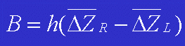
where h = hemisphere (1 = NH, -1 = SH).
DeltaZR = mean 900-600hPa thickness in semicircle right of motion
DeltaZL = mean 900-600hPa thickness in semicircle left of motion
The mean thicknesses are evaluated in semicircles of radius 500km.
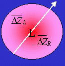
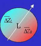
This parameter measures the strength of the frontal nature of the cyclone. Three examples of varying magnitudes of B are shown below.
 B = 0
The example to the left illustrates a near-zero value of B. The magnitude of B is calculated as the difference in thickness (shaded) between the semicircle right of motion from that left of motion. A value near zero for B indicates a nonfrontal cyclone. The example to the left is a schematic for a conventional tropical cyclone, which has a maximum of thickness in the center of the cyclone that decreases almost uniformly outward in all directions.
B = 0
The example to the left illustrates a near-zero value of B. The magnitude of B is calculated as the difference in thickness (shaded) between the semicircle right of motion from that left of motion. A value near zero for B indicates a nonfrontal cyclone. The example to the left is a schematic for a conventional tropical cyclone, which has a maximum of thickness in the center of the cyclone that decreases almost uniformly outward in all directions.
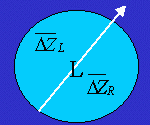 B = 0
The example to the left also illustrates a near-zero value of B. This schematic example is for an occluded extratropical cyclone.
B = 0
The example to the left also illustrates a near-zero value of B. This schematic example is for an occluded extratropical cyclone.
 B >> 0
The example to the left illustrates a positive value of B. The semicircle right of motion has a substantially larger thickness (warmer) than that left of motion. Thus, this schematic represents a frontal cyclone with strong temperature gradients perpendicular to the storm motion. This schematic is for a conventional intensifying or mature extratropical cyclone.
B >> 0
The example to the left illustrates a positive value of B. The semicircle right of motion has a substantially larger thickness (warmer) than that left of motion. Thus, this schematic represents a frontal cyclone with strong temperature gradients perpendicular to the storm motion. This schematic is for a conventional intensifying or mature extratropical cyclone.
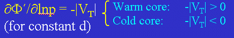
- "-VTL" - The magnitude of the cyclone lower troposphere thermal wind. This is measured as the vertical profile of cyclone geopotential height gradient (cyclone strength) between 900 and 600hPa.
This second parameter measures the fundamental cold, neutral, or warm core structure of the cyclone in the lower-middle troposphere.
Thermal wind dictates that cyclone phase is related to cyclone strength profile:
- A warm core cyclone has a profile of cyclone strength that decreases with height.
- A cold core cyclone has a profile of cyclone strength that increases with height.
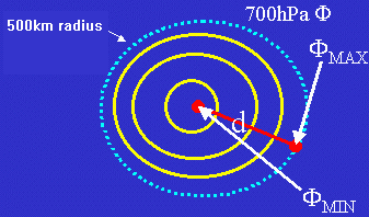
- Cyclone strength is measured as the height perturbation, phi'.
- phi' = phiMAX - phiMIN
- This difference approximates the height gradient on an isobaric surface and the magnitude of the geostrophic wind (Vg).
- phi' = df|Vg|/g
- where d = distance between extrema, g = gravity, and f = coriolis parameter.
The cyclone's full 3-D structure is given by the vertical derivative of phi', which is the thermal wind (VT):
- "-VTU" - This is the same as (2), except is calculated for the middle/upper troposphere -- between 600 and 300hPa. This gives the measure of cyclone phase (cold vs warm core) for the upper troposphere. This third measures helps to distinguish full-troposphere warm-core cyclones (e.g. tropical cyclones) from shallow warm core cyclones (warm-seclusions or subtropical cyclones).
Note that although cold-core cyclones typically tilt (westward) with height, thermal wind is still calculated in a vertical column and the calculations here are still valid for tilting cyclones.
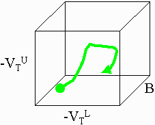 These three parameters, B, -VTL, and -VTU represent each of three dimensions of the experimental cyclone phase space. In reality, there are many more dimensions of cyclone phase (larger scale flow, stratospheric interaction, surface fluxes, etc); however, the three chosen here represent the majority of the variability among known synoptic-scale cyclones.
Since a 3-D cube of cyclone phase space is difficult to visualize and interpret in real-time, the cyclone phase is plotted using two cross sections through the cube:
2. Phase Diagram #1 Construction: B Vs. -VT
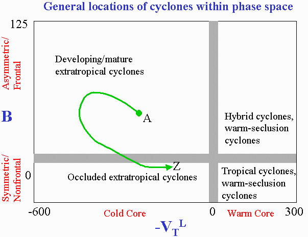
- The vertical axis of the phase diagram is represented by the parameter "B".
- The horizontal axis of the phase diagram is represented by the parameter "-VTL".
- Four generic quadrants of cyclone type result:
- Frontal/asymmetric warm-core [TR]
- Nonfrontal/symmetric warm-core [BR]
- Nonfrontal/symmetric cold-core [BL]
- Frontal/asymmetric cold-core [TL]
- The conventional types of cyclones can be labeled within the phase space, although past and current research have shown there are no hard boundaries between each of the cyclone types.
- The full cyclone lifecycle (past, current, and/or forecast) can be plotted within the phase space (note schematic green arrow in example to the left).
- The start of the cyclone in the online database is labeled by 'A' and the end of the cyclone in the online database (end of forecast time, or decay, whichever is reached first), is labeled by 'Z'.
3. Phase Diagram #2 Construction: -VTL Vs. -VTU

- The vertical axis of the phase diagram is represented by the parameter "-VTU".
- The horizontal axis of the phase diagram is represented by the parameter "-VTL".
- Four generic quadrants of cyclone type result:
- Full troposphere warm core [TR]
- Lower warm core, upper cold-core [BR]
- Full troposphere cold core [BL]
- Lower cold core, upper warm-core [TL]
- The conventional types of cyclones can be labeled within the phase space, although past and current research
have shown there are no hard boundaries between each of the cyclone types.
- The full cyclone lifecycle (past, current, and/or forecast) can be plotted within the phase space (note schem
atic green arrow in example to the left).
- The start of the cyclone in the online database is labeled by 'A' and the end of the cyclone in the online da
tabase (end of forecast time, or decay, whichever is reached first), is labeled by 'Z'.
4. Actual phase diagrams
Additional information provided on the actual diagrams include:
- The model type and initialization time for the cyclone is labeled on top.
- If the cyclone already exists, a 'C' is used to identify the current location on the cyclone evolution path.
- If the cyclone phase line and markers are solid, it indicates history (past analyses); if the line and markers are dotted, it indicates the model forecast.
- During the phase evolution, the 00Z times are labeled with the two-digit date.
- The color of the line and marker indicate the cyclone intensity (minimum SLP).
- The marker size represents the size of the 925hPa wind field (mean radius).
- The corresponding current model analysis of SLP and SST are shown in the upper
right inset frame.
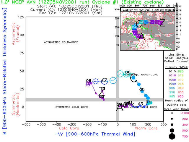
Phase Diagram #1 Example:
Phase Diagram #2 Example:
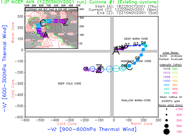
Interpretation of these example diagrams:
- These diagrams are for the formation, extratropical transition, and occlusion of Hurricane Michelle (2001), as analyzed and forecast by the NCEP AVN model.
- The cyclone was first analyzed (closed SLP field < 1018hPa) at 1800 UTC 25 October 2001, as labeled by the 'A'.
- The latest analysis, as labeled by the 'C', is 1200 UTC 5 November 2001.
- The solid circles within the phase diagrams indicate the classic 900-300hPa symmetric warm-core development and amplification through 4 November.
- Extratropical transition begins 1800 UTC 4 November, when the value of B exceeds 10m.
- At the current analysis time (1200 UTC 5 November 2001), extratropical transition is continuing, with the cyclone diagnosed as a strong warm-core yet highly frontal cyclone below 600hPa, and an increasingly cold core structure above 600hPa.
- The size of the gale force wind field at 925hPa is forecast to continue expanding in size, to nearly 650km, consistent with other cases of extratropical transition.
- The latest AVN forecast completes extratropical transition at 1800 UTC 6 November (when -VTL becomes negative). The cyclone then
weakens and occludes on 10 November.
4. Frequently Asked Questions
- Why should we be concerned with cyclone phase?
Understanding the phase of cyclones gives a broader, yet insightful, perspective on the overwhelming distribution of all cyclones. Cyclones aren't simply tropical or extratropical; there is a great continuum of cyclone types, with a significant fraction of them having characteristics of both tropical and extratropical cyclones.
The phase of a cyclone (warm vs cold-core, in particular) is related to its intensity, size, forecast uncertainty, and ultimately the threat it poses to us. Generally, a warm core cyclone has more forecast uncertainty associated with it than a cold-core cyclone. For example, the development and intensification of tropical cyclones is one of the most difficult forecasts to make. The diagnostics shown here give an indiciation of whether a cyclone that is developing within the models is a pure warm-core development, or hybrid development.
Forecasting the phase conversion or transition of cyclones (e.g. tropical into extratropical and subtropical into tropical) is a difficult but important task, and the phase diagnoses provided here provide considerable insight into the essence of model cyclone development. In concert with real-time surface, ship, and satellite observations, a more accurate diagnosis and forecast of cyclone evolution is possible when the phase diagrams are used.
During the 2001 hurricane season, the phase diagnoses provided here accurately forecast the conversion of two subtropical cyclones into Hurricanes Karen and Olga. The extratropical transition of Hurricanes Gabrielle and Michelle were both well-forecast by the phase diagrams as well.
These diagrams also provide for forecast track and intensity comparison.
- What models are available for phase analysis? Why isn't the ECMWF available?
NCEP AVN, Eta and NGM; U.S. Navy NOGAPS; U.S. Air Force MM5; Canadian Meteorological Center Global CMC; UK Met Office UKMET. The ECMWF model data available to us is (unfortunately) far too coarse to allow reliable phase analysis.
- Why aren't all the closed SLP minima on the model analyses available for phase diagram analysis?
A cyclone will not be analyzed on the phase diagrams if: 1) the cyclone is currently too close to the edge of the model domain, 2) the cyclone does not last for 24h, or 3) the cyclone has a minimum SLP > 1018mb.
- Why are some cyclones labeled as red and others as black?
The black ones are existing cyclones, the red ones are forecast cyclones that have not yet developed.
- Why do many of the cyclones only show current and forecast analysis (not past)?
Either the cyclone has just formed, has not yet formed, or the database has a large gap in it from missing data that has prevented continuous tracking of the cyclone from one model analysis to the next.
- Why is there a sudden jump in the track of a cyclone/Why does a cyclone track suddenly end even though it has not decayed?
The detection of cyclones and tracking them is a very complex and difficult process. Cyclones may form downstream from an already existing cyclone. In this case, it can become difficult to determine where the path of one cyclone ends and another begins. As a result, the track and phase evolution of a cyclone can appear to jump, if another, stronger, cyclone forms relatively close to an existing cyclone. Also, if a cyclone moves extremely quickly (> 30 ms-1), the tracking algorithm may interpret the new cyclone position as the formation of a new cyclone. This is most likely in the NOGAPS, UKMET, and CMC analyses which are available only every 12h -- and, consequently, large changes in cyclone position can result.
- What is the model intercomparison format?
Thumbnail versions of the phase diagrams for a given cyclone are compared, allowing the user to compare the current and forecast phase evolution for a single cyclone among several models. Note that not all models will necessary resolve the same cyclones, especially in the tropics. The consensus forecast (unweighted mean of all available models) for the given cyclone is also presented. The 1 standard deviation variability from this mean is given as the shading either side of the mean phase analysis.
- Why aren't cyclones near high terrain analyzed?
The two parameters used to describe the cyclones (B, -VT) are calculated over the pressure ranges of 900-600hPa. If high terrain enters this pressure range, then the field values for thickness and geopotential height are contaminated by interpolation below ground. As a result, the diagnostics are not representative of the atmosphere or the cyclone's true phase, and it will not be analyzed.
- Why are cyclones analyzed only for the western Hemisphere north of the equator?
Existing computer resources do not allow us to examine the entire globe.
- Satellite shows that a tropical storm CLEARLY exists at location X, yet the phase diagrams are showing only a marginal warm core structure at best!
The phase analyses shown here are derived completely from model analyses and forecasts. They will not and cannot represent the complete or true structure of the observed cyclone. The phase diagrams are only as accurate as the model analyses and forecasts from which they are derived. As model analyses become increasingly more accurate, so will the phase diagrams.
5. Relevant/helpful references
Hart, R.E., 2003: A cyclone phase space derived from thermal wind and thermal asymmetry. Mon. Wea. Rev., 131, 585-616.
Evans, J.L. and R. Hart, 2003: Objective indicators of the extratropical transition lifecycle of
Atlantic tropical cyclones. Mon. Wea. Rev., 131, 909-925.
Beven, J.L. II, 1997: A Study of Three "Hybrid" Storms. Proc. 22nd Conf. on Hurricanes and Tropical Meteorology, Fort Collins, CO. Amer. Meteor. Soc., 645-646.
Miner, T., P. J. Sousounis, J. Wallman, and G. Mann, 2000: Hurricane Huron. Bulletin of the American Meteorological Society. 81, 223-236.
Last Updated: 18 February 2003